In this chapter, we will discuss shell loop control in Unix. So far you have looked at creating loops and working with loops to accomplish different tasks. Sometimes you need to stop a loop or skip iterations of the loop.

In this chapter, we will learn the following two statements that are used to control shell loops−

• The break statement
• The continue statement

The infinite Loop

All the loops have a limited life and they come out once the condition is false or true depending on the loop.

A loop may continue forever if the required condition is not met. A loop that executes forever without terminating executes for an infinite number of times. For this reason, such loops are called infinite loops.

Example

Here is a simple example that uses the while loop to display the numbers zero to nine −

#!/bin/sh

a=10

until [ $a -lt 10 ]
do
   echo $a
   a=`expr $a + 1`
done

This loop continues forever because a is always greater than or equal to 10 and it is never less than 10.

The break Statement

The break statement is used to terminate the execution of the entire loop, after completing the execution of all of the lines of code up to the break statement. It then steps down to the code following the end of the loop.

Syntax

The following break statement is used to come out of a loop −

break

The break command can also be used to exit from a nested loop using this format −

break n

Here n specifies the n^th enclosing loop to the exit from.

Example

Here is a simple example that shows that the loop terminates as soon as a becomes 5 −

#!/bin/sh

a=0

while [ $a -lt 10 ]
do
   echo $a
   if [ $a -eq 5 ]
   then
      break
   fi
   a=`expr $a + 1`
done

Upon execution, you will receive the following result −

0
1
2
3
4
5

Here is a simple example of a nested for loop. This script breaks out of both loops if var1 equals 2 and var2 equals 0 

#!/bin/sh

for var1 in 1 2 3
do
   for var2 in 0 5
   do
      if [ $var1 -eq 2 -a $var2 -eq 0 ]
      then
         break 2
      else
         echo "$var1 $var2"
      fi
   done
done

Upon execution, you will receive the following result. In the inner loop, you have a break command with argument 2. This indicates that if a condition is met you should break out of the outer loop and ultimately from the inner loop as well.

1 0
1 5

The continue statement

The continue statement is similar to the break command, except that it causes the current iteration of the loop to exit, rather than the entire loop.

This statement is useful when an error has occurred but you want to try to execute the next iteration of the loop.

Syntax

continue

Like with the break statement, an integer argument can be given to the continue command to skip commands from nested loops.

continue n

Here n specifies the n^th enclosing loop to continue from.

Example

The following loop makes use of the continue statement which returns from the continue statement and starts processing the next statement

#!/bin/sh

NUMS="1 2 3 4 5 6 7"

for NUM in $NUMS
do
   Q=`expr $NUM % 2`
   if [ $Q -eq 0 ]
   then
      echo "Number is an even number!!"
      continue
   fi
   echo "Found odd number"
done

Upon execution, you will receive the following result −

Found odd number
Number is an even number!!
Found odd number
Number is an even number!!
Found odd number
Number is an even number!!
Found odd number

In this chapter, we will discuss shell loops in Unix. A loop is a powerful programming tool that enables you to execute a set of commands repeatedly. In this chapter, we will examine the following types of loops available to shell programmers −

• The while loop
• The for loop
• The until loop
• The select loop

You will use different loops based on the situation. For example, the while loop executes the given commands until the given condition remains true; the until loop executes until a given condition becomes true.

Once you have good programming practice you will gain the expertise and thereby, start using appropriate loops based on the situation. Here, while and for loops are available in most of the other programming languages like C, C++, PERL, etc.

Nesting Loops

All the loops support the nesting concept which means you can put one loop inside another similar one or different loops. This nesting can go up to an unlimited number of times based on your requirement.

Here is an example of a nesting while loop. The other loops can be nested based on the programming requirement in a similar way −

Nesting while Loops

It is possible to use a while loop as part of the body of another while loop.

Syntax

while command1 ; # this is loop1, the outer loop
do
   Statement(s) to be executed if command1 is true

   while command2 ; # this is loop2, the inner loop
   do
      Statement(s) to be executed if command2 is true
   done

   Statement(s) to be executed if command1 is true
done

Example

Here is a simple example of loop nesting. Let’s add another countdown loop inside the loop that you used to count to nine −

#!/bin/sh

a=0
while [ "$a" -lt 10 ]    # this is loop1
do
   b="$a"
   while [ "$b" -ge 0 ]  # this is loop2
   do
      echo -n "$b "
      b=`expr $b - 1`
   done
   echo
   a=`expr $a + 1`
done

This will produce the following result. It is important to note how echo -n works here. Here -n option lets echo avoid printing a new line character.

0
1 0
2 1 0
3 2 1 0
4 3 2 1 0
5 4 3 2 1 0
6 5 4 3 2 1 0
7 6 5 4 3 2 1 0
8 7 6 5 4 3 2 1 0
9 8 7 6 5 4 3 2 1 0

Are you a web developer, who does create amazing websites but doesn’t know much about all the theoretical concepts like software design patterns, and all? Today, let’s understand the two basic types of software development patterns, primarily used in web development frameworks.

Let’s see what MVC (Model View Controller) and MVT (Model View Template) design patterns are and the differences between them. MVC and MVT patterns allow developers to change the visual part of an app and the business logic part separately.

If you have come here to know the differences between these patterns, and you aren’t patient enough to read the entire article, here is a quick answer for you.

What is the difference between MVC and MVT? In MVC, programmers need to write all the control-specific code whereas, in MVT, the framework itself handles the controller part. There are also some differences when it comes to the presentation of data to the user.

I know you won’t understand much from this quick answer if you are a beginner at these concepts. So, let’s deep dive into both design patterns and understand them.

Model View Controller (MVC)

This design pattern breaks down software into three major components: the model, the view, and the controller. Each of these components has independent jobs, and they can work separately without affecting each other.

Let’s see the role of each component in MVC.

• Model – The model represents an object carrying data. It can also have logic to update the controller if its data changes. But, it contains no logic describing how to present the data to a user.
• View – View represents the visualization of the data that the model contains. The view knows how to access the model’s data, but it does not know what this data means.
• Controller – The controller acts on both model and view. It controls the data flow into the model object and updates the view whenever data changes. It keeps the view and model separate.

This is done to separate internal representations of information from the ways information is presented to and accepted by the user.

The main advantage of using a design pattern like this is that multiple developers can work simultaneously on each of these specific components.

The best thing about MVC is that each component has a particular purpose. The model part holds the data of your app, the View makes your app look pretty, and the Controller controls how your app functions. Any web application is structured, keeping these three core components in mind.

MVC helps to organize the core functions of your code neatly. It will be easy to make any changes to your app later as you will be able to identify which code does what.

Also, if you’re using an MVC framework, then it will be easy to share your code with other developers. After the initial learning hurdle, everything becomes easy when you use a framework.

MVC reduces complexities in designing web apps, primarily large applications, by keeping the code and workflow structured. It makes the overall code simple to maintain, test, debug, and reuse.

You can watch the following video to learn more about MVC.

Model View Template (MVT) 

The Model-View-Template (MVT) is slightly different from MVC. It is a collection of three essential components Model, View, and Template. These three layers are responsible for different things, and we use them independently. Django is a popular web development framework that uses the MVT design pattern. 

The main difference between the two patterns is that Django itself takes care of the Controller part (Software Code that controls the interactions between the Model and View), leaving us with the template. The template is an HTML file mixed with Django Template Language (DTL).

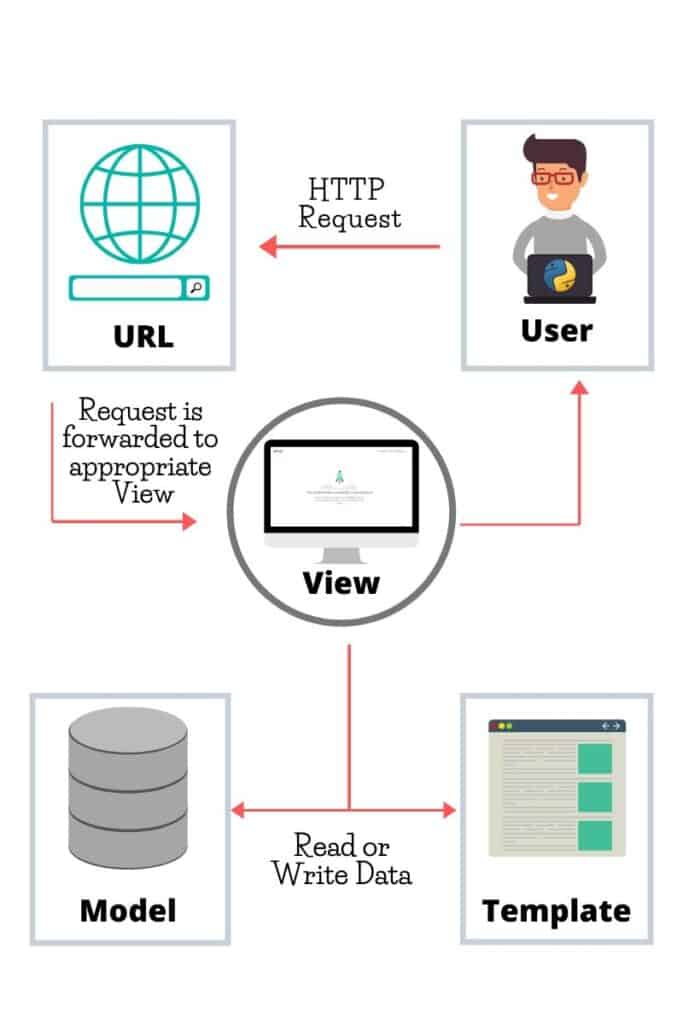
Here is a simple diagram that shows the MVT architecture in Django:

So, in the case of Django, let’s see what each component is doing:

• The model helps to handle the database. It is a data access layer, which contains the required fields and behaviors of the data you’re storing. There’s hardly an application without a database. A model is a Python class, and it does not know anything about other Django layers.  Models help developers to create, read, update, and delete objects (CRUD operations) in the original database. Also, they hold business logic, custom methods, properties, and other things related to data manipulation.
• The view is used to execute the business logic and interact with a model to carry data and render a template. The view fetches data from a model. Then, it either gives each template access to specific data to be displayed, or it processes data beforehand. It accepts HTTP requests, applies business logic provided by Python classes and methods, and provides HTTP responses to the client requests.
• The template is a presentation layer that handles the User Interface part completely. These are files with HTML code, which is used to render data. The contents of these files can be static or dynamic. A template is used only to present data since there’s no business logic in it.

In Django, the view describes which data is presented, but a view normally delegates to a template, which describes how the data is presented.

The developer provides the model, the view, and the template, then maps it to a URL, and Django does the magic, to serve it to the user.

In short, a web application has data, layout, and logic. The model will work with the data, the view will work with the logic, and the template will work with the layout.

If you’re familiar with other MVC Web-development frameworks, you may consider Django views to be the controllers and Django templates to be the views.

In Django, the view describes the data that gets presented to the user; it’s not necessarily how the data looks, but which data gets presented.

The view describes which data you see, not how you see it. It’s a subtle distinction. Also, it’s sensible to separate content from presentation – which is where templates come in.

The controller is the framework itself, the machinery that sends a request to the appropriate view, according to the Django URL configuration. [Source].

At the end of the day, it comes down to getting stuff done. Also, regardless of how things are named, Django gets stuff done most logically.

So, that’s all about the differences between MVC and MVT design patterns.

If you have any doubts regarding this, leave them in the comments section below. I’ll be happy to help you. Also, if you have any additional points to make regarding this topic, let me know in the comments.

If you’re looking to do your next project using the Django framework, I want you to check out this resource. I’ve written an article that lists out 12 Django Project Ideas that you can take and implement right away.

If this article was helpful, do share this article with your fellow programmers. I would appreciate it, and it will encourage me to create more useful tutorials like this.

Happy coding!